While we have explored some basic applications of exponential and logarithmic functions, in this section we explore some important applications in more depth.
In an earlier section, we discussed radioactive decay - the idea that radioactive isotopes change over time. One of the common terms associated with radioactive decay is half-life.
Given the basic exponential growth/decay equation \(h(t)=ab^{t}\text{,}\) half-life can be found by solving for when half the original amount remains; by solving \(\dfrac{a}{2}=a(b)^{t}\text{,}\) or more simply \(\dfrac{1}{2}=b^{t}\text{.}\) Notice how the initial amount is irrelevant when solving for half-life.
We were not given a starting quantity, so we could either make up a value or use an unknown constant to represent the starting amount. To show that starting quantity does not affect the result, let us denote the initial quantity by the constant \(a\text{.}\) Then the decay of Bismuth-210 can be described by the equation \(Q(d)=a(0.87)^{d}\text{,}\) where \(d\) is a number of days.
To find the half-life, we want to determine when the remaining quantity is half the original: \(\dfrac{a}{2}\text{.}\) We start by setting our function equal to this desired output: \(\dfrac{a}{2}=a(0.87)^{d}\text{.}\) Then we divide both sides of the equation by \(a\) to get \(\dfrac{1}{2}=0.87^{d}\text{.}\) We can then take the common log of both sides to get \(\log(\dfrac{1}{2})=\log(0.87^{d})\text{,}\) and then use the exponent property of logs to find \(\log(\dfrac{1}{2})=d\log(0.87)\text{.}\) Dividing to solve for \(d\) gives us \(d=\dfrac{\log(\dfrac{1}{2})}{\log(0.87)}\approx 4.977 \text{ days}\text{.}\)
Since we are looking for an annual decay rate, we will use an equation of the form \(Q(t)=a(1+r)^{t}\text{.}\) We know that after 30 years, half the original amount will remain. Using this information, we can write the equation \(\dfrac{a}{2}=a(1+r)^{30}\text{.}\) Dividing both sides by a gives us \(\dfrac{1}{2}=(1+r)^{30}\text{.}\) Taking the 30th root of both sides gives us \((\dfrac{1}{2})^{\frac{1}{30}}=1+r\text{,}\) and then subtracting one from both sides gives us \(r=(\dfrac{1}{2})^{\frac{1}{30}}-1\approx -0.02284\text{.}\)
Carbon-14 is a radioactive isotope that is present in organic materials, and is commonly used for dating historical artifacts. Carbon-14 has a half-life of 5730 years. If a bone fragment is found that contains 20% of its original carbon-14, how old is the bone?
To find how old the bone is, we first will need to find an equation for the decay of the carbon-14. We could either use a continuous or annual decay formula, but opt to use the continuous decay formula since it is more common in scientific texts. The half life tells us that after 5730 years, half the original substance remains. Solving for the rate, \(\dfrac{a}{2}=ae^{5730r}\text{.}\) Dividing by a gives us \(\dfrac{1}{2}=e^{5730r}\text{,}\) and then taking the natural log of both sides gives \(\ln(\dfrac{1}{2})=\ln(e^{5730r})\text{.}\) Use the inverse property of logs on the right side to get \(\ln(\dfrac{1}{2})=5730r\text{.}\) Then we can divide by 5730 to see \(r=\dfrac{\ln(\frac{1}{2})}{5730}\approx -0.000121\text{.}\)
Now we know the decay will follow the equation \(Q(t)=ae^{-0.000121t}\text{.}\) To find how old the bone fragment is that contains 20% of the original amount, we solve for \(t\) so that \(Q(t) = 0.20a\text{.}\)
Our initial equation to set up should look like \(0.20a=ae^{-0.000121t}\text{.}\) Then we divide by \(a\) to get \(0.20=e^{-0.000121t}\text{,}\) and then take the natural log of both sides to get \(\ln( 0.20)=\ln(e^{-0.000121t})\text{.}\) The inverse property reduces the right hand side, giving us \(\ln(0.20)=-0.000121t\text{,}\) and we can divide to solve for \(t\) to find \(t=\dfrac{\ln( 0.20)}{-0.000121}\approx 13301 \text{ years}\text{.}\)
We have already learned that Cesium-137 has a half-life of about 30 years. If you begin with 200 mg of cesium-137, will it take more or less than 230 years until only 1 milligram remains?
For decaying quantities, we asked how long it takes for half the substance to decay. For growing quantities we might ask how long it takes for the quantity to double.
Given the basic exponential growth equation \(h(t)=ab^{t}\text{,}\) doubling time can be found by solving for when the original quantity has doubled; by solving \(2a=a(b)^{x}\text{,}\) or more simply \(2=b^{x}\text{.}\) Like with decay, the initial amount is irrelevant when solving for doubling time.
Cancer cells sometimes increase exponentially. If a cancerous growth contained 300 cells last month and 360 cells this month, how long will it take for the number of cancer cells to double?
Defining \(t\) to be time in months, with \(t = 0\) corresponding to last month, we are given two pieces of data: last month, \((0, 300)\text{,}\) and this month, \((1, 360)\text{.}\)
From this data, we can find an equation for the growth. Using the form \(C(t)=ab^{t}\text{,}\) we know immediately \(a = 300\text{,}\) giving \(C(t)=300b^{t}\text{.}\) Substituting in \((1, 360)\text{,}\) we see \(360=300b^{1}\text{,}\) and so \(b\dfrac{360}{300}=1.2\text{.}\)
To find the doubling time, we look for the time when we will have twice the original amount, so when \(C(t) = 600\text{.}\) Our starting equation is \(600=300(1.2)^{t}\text{.}\) Dividing by 300 gives us \(2=(1.2)^{t}\text{,}\) and we can then take the common log of both sides to see \(\log(2)=\log(1.2^{t} )\text{.}\) The exponential property gives us the equation \(\log(2)=t\log(1.2)\text{,}\) and we can divide both sides by \(\log(1.2)\) to get \(t=\dfrac{\log(2)}{\log(1.2)}\approx 3.802\text{.}\) So it will take about 3.802 months for the number of cancer cells to double.
Use of a new social networking website has been growing exponentially, with the number of new members doubling every 5 months. If the site currently has 120,000 users and this trend continues, how many users will the site have in 1 year?
We can use the doubling time to find a function that models the number of site users, and then use that equation to answer the question. While we could use an arbitrary \(a\) as we have before for the initial amount, in this case, we know the initial amount was 120,000.
If we use a continuous growth equation, it would look like \(N(t)=120e^{r}t\text{,}\) measured in thousands of users after \(t\) months. Based on the doubling time, there would be 240 thousand users after 5 months. This allows us to solve for the continuous growth rate: \(240=120e^{5r}\text{,}\) so \(2=e^{5r}\text{.}\) Then, \(\ln(2)=5r\text{,}\) and so \(r=\dfrac{\ln(2)}{5}\approx 0.1386\text{.}\)
Now that we have an equation, \(N(t)=120e^{0.1386t}\text{,}\) we can predict the number of users after 12 months: \(N(12)=120e^{0.1386(12)}=633.140 \text{ thousand users}\text{.}\)
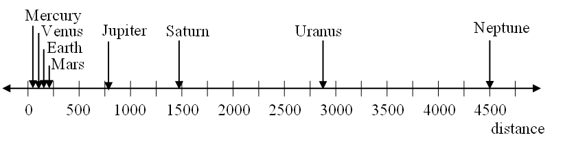
For quantities that vary greatly in magnitude, a standard scale of measurement is not always effective, and utilizing logarithms can make the values more manageable. For example, if the average distances from the sun to the major bodies in our solar system are listed, you see they vary greatly.
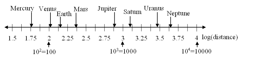
However, computing the logarithm of each value and plotting these new values on a number line results in a more manageable graph, and makes the relative distances more apparent.
Sometimes, as shown above, the scale on a logarithmic number line will show the log values, but more commonly the original values are listed as powers of 10, as shown below.
Notice that on the log scale above, the visual distance on the scale between points \(A\) and \(B\) is the same as the distance between points \(C\) and \(D\text{.}\) When looking at the values these points correspond to, notice \(B\) is ten times the value of \(A\text{,}\) and \(D\) is ten times the value of \(C\text{.}\) A visual linear difference between points corresponds to a relative (ratio) change between the corresponding values.
Logarithms are useful for showing these relative changes. For example, comparing $1,000,000 to $10,000, the first is 100 times larger than the second. That is, \(\dfrac{1000000}{10000}=100=10^{2}\text{.}\)
When one quantity is roughly ten times larger than another, we say it is one order of magnitude larger. In both cases described above, the first number was two orders of magnitude larger than the second.
Notice that the order of magnitude can be found as the common logarithm of the ratio of the quantities. On the log scale above, \(B\) is one order of magnitude larger than \(A\text{,}\) and \(D\) is one order of magnitude larger than \(C\text{.}\)
Given two values \(A\) and \(B\text{,}\) to determine how many orders of magnitude \(A\) is greater than \(B\text{,}\)\(\text{Difference in orders of magnitude}= \log(\dfrac{A}{B})\)
The relative change is \(\dfrac{100,000}{100}=1000=10^{3}\text{.}\) The log of this value is 3. Thus, \(C\) is three orders of magnitude greater than \(B\text{,}\) which can be seen on the log scale by the visual difference between the points on the scale.
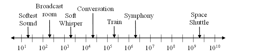
Using the table from the previous exercise, what is the difference of order of magnitude between the softest sound a human can hear and the launching of the space shuttle?
An example of a logarithmic scale is the Moment Magnitude Scale (MMS) used for earthquakes. This scale is commonly and mistakenly called the Richter Scale, which was a very similar scale succeeded by the MMS.
If one earthquake has a MMS magnitude of 6.0, and another has a magnitude of 8.0, how much more powerful (in terms of earth movement) is the second earthquake?
Since the first earthquake has magnitude 6.0, we can find the amount of earth movement for that quake, which we’ll denote \(S_{1}\text{.}\) The value of \(S_{0}\) is not particularly relevant, so we will not replace it with its value. We start solving for \(S_{1}\) by setting up the equation \(6.0=\dfrac{2}{3}\log(\dfrac{S_1}{S_0})\text{.}\) Continuing to solve for \(S_{1}\text{,}\) we see:
Doing the same with the second earthquake, \(S_{2}\text{,}\) with a magnitude of 8.0, the equation \(8.0=\dfrac{2}{3}\log(\dfrac{S_2}{S_0})\) gives us \(S_{2}=10^{12}S_{0}\text{.}\)
One earthquake has magnitude of 3.0. If a second earthquake has twice as much earth movement as the first earthquake, find the magnitude of the second quake.
In fact, using log properties, we could show that whenever the earth movement doubles, the magnitude will increase by about 0.201. Given the movement of an earthquake denoted by \(S\text{,}\) the magnitude of a second earthquaqe with twice the movement is:
Since \(\dfrac{2}{3}\log(\dfrac{S}{S_0})\) is the magnitude of the first earthquake, the magnitude of the second is 0.201 greater than the magnitude of the first.
This illustrates the most important feature of a log scale: that multiplying the quantity being considered will add to the scale value, and vice versa.
Solving \(a(1+0.066)^{t}=2a\text{,}\) it will take \(t=\dfrac{\log(2)}{\log(1.066)}\approx 10.845 \text{ years}\text{,}\) or approximately 11 years, for tuition to double.
\(\dfrac{2\times10^9}{2\times10^1}=10^{8}\text{.}\) The sound pressure in created by launching the space shuttle is 8 orders of magnitude greater than the sound pressure created by the softest sound a human ear can hear.